Home » Improving crop modeling using machine learning

Improving crop modeling using machine learning

Integration of machine learning and crop modelling can optimize predictions of plant growth and yield.

The page can be listened to as an audio file.

As climate change intensifies, scientists are working to find the best performing methods, algorithms, or models to simulate the impact of high temperature and/or limited water availability on crop growth, development and productivity. The complexity of plant-environment interactions makes this difficult, but new research has shown that the integration of machine learning and crop modelling may provide the answers needed.

Dr. Ioannis Droutsas, Research Fellow at the University of Leeds, and coauthors embedded machine learning (ML) algorithms into a process-based crop model to create a new crop modelling/ML framework with high performance in the representation of crop response to a wide range of environments,  including stress conditions.

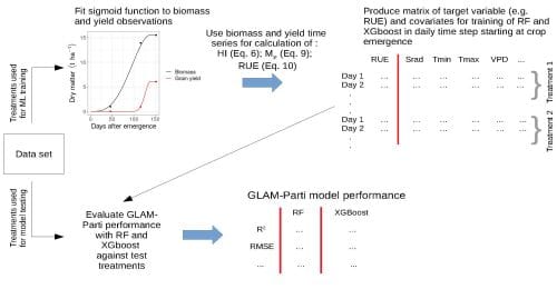
The authors modified the existing process-based crop model GLAM-Parti  by embedding  machine learning algorithms  to estimate variables that regularly escape the crop model’s predictive capacity. .  ML was used for daily predictions of radiation use efficiency, the rate of change of harvest index and the phenological stage.

For the assessment of the new GLAM-Parti-ML framework, the authors used an existing data set for one cultivar of wheat grown under a wide range of temperatures, solar radiation, and atmospheric humidity conditions, including exposure to heat stress. Half of the data was used to train the machine learning algorithms and the other half to test the model.

The model was run with the weather inputs temperature, solar radiation and vapor pressure deficit, the most significant weather determinants of wheat growth for irrigated, well fertilized conditions. The outputs of biomass and grain yield, as well as the days to anthesis and maturity were compared to the end-of-season field measurements.

A flow chart showing the methodology for integration of ML into GLAM-Parti. The data set is split into training and testing treatments. Crop data from the training treatments are used for fitting time-series of biomass and yield, which then derive the target variables RUE and dHI/dt for training of Random Forests (RF) and XGBoost. The test treatments are used in the evaluation of GLAM-Parti with RF and XGBoost respectively.
Methodology for integration of ML into GLAM-Parti.

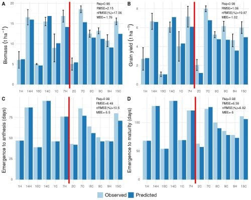
The team applied Random Forests and Extreme Gradient Boosting. Both ML models exhibited high efficiency in learning the patterns between inputs and crop performance (in terms of radiation use efficiency) during the course of the growing season. This resulted in good model skill for crop biomass; GLAM-Parti-ML reproduced 98% of the observed variance in both biomass and grain yield and the model error was less than 20%. Moreover, the model reproduced at least 98% of the observed variance in the days to anthesis and maturity with less than 11% error. Nevertheless, the onset of both phenological stages was underestimated, thus predicting anthesis and maturity earlier than observed.

Four figures are shown. The paired barcharts compare observed and predicted biomass, grain yield, emergence to anthesis and emergence to maturity dates. All have 12 cultivars listed on the x axis and a red vertical line in the center indicating that 6 of the cultivars are used training of Random Forests and the other 6 are treatments used for model testing. The y-axis for figure A is biomass in tons per hectare from 0-20. The biomass for three of the training cultivars and one testing cultivar is around 5 tones per hectare, while the value for other cultivars is around 10 tons per hectare. The training prediction values are over- and under-estimated evenly while the testing values show predictions to be underestimated. 
The y-axis for figure B is grain yield in tons per hectare from 0-8. The biomass for two of the training cultivars and one testing cultivar is around 1 ton per hectare, while the value for other cultivars is around 5 tons per hectare. The training prediction values are over- and under-estimated evenly while the testing values show predictions to be underestimated.
The y-axis for figure C is emergence to anthesis from 0-100 days. The anthesis date varies for both the training and testing cultivars and range from 50-100 days. The training prediction values are equal to the observed values while the testing values show predictions to be underestimated.
The y-axis for figure D is emergence to maturity from 0-150 days. The maturity date varies for both the training and testing cultivars and range from 75-150 days. The training prediction values are equal to the observed values while the testing values show predictions to be mostly underestimated.
Comparison between observed and GLAM-Parti simulated values for one cultivar of wheat grown under a wide range of temperatures, solar radiation, and atmospheric humidity conditions, including exposure to heat stress. Vertical red lines separate the treatments used for training of Random Forests (left of red line) and the treatments used for model testing (right of red line).

Next, GLAM-Parti was compared to its predecessor, GLAM, a process-based crop model with no integration of machine learning.  GLAM was calibrated with 100% of the data and GLAM-Parti with only 50%. Nevertheless, GLAM-Parti-ML had lower error values for biomass, yield, and the days to maturity and anthesis, indicating that the machine learning parameterizations improved the model despite being trained on only half of the data.

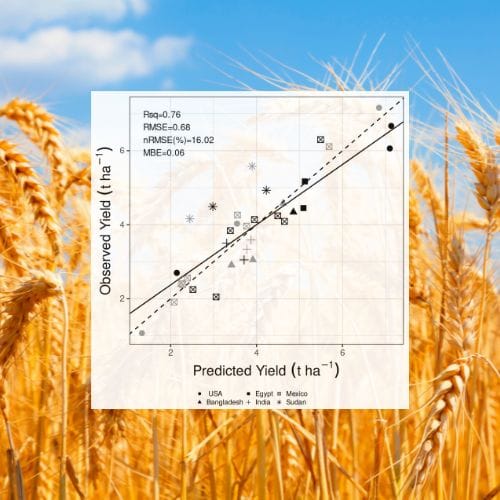
To further evaluate GLAM-Parti-ML, the authors used a second data set of three cultivars of wheat grown in many field experiments across six countries. Again, half of the data was used to train the machine learning algorithms and the other half to test the model.

Four figures are shown. The scatter plots compare observed and predicted biomass, grain yield, emergence to anthesis and emergence to maturity dates for wheat grown in 4 countries. 
The axes for figure A are biomass in tons per hectare from 0-15. The R squared value is 0.73. 
The y axes for figure B are grain yield in tons per hectare from 0-7.5. The R squared value is 0.76.
The axes for figure C are emergence to anthesis from 0-100 days. The R squared value is 0.66.
The axes for figure are is emergence to maturity from 0-120 days. The R squared value is 0.79.
Comparison between observed and GLAM-Parti simulated values for three cultivars of wheat grown in many field experiments across six countries.

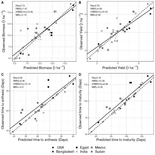
Once more, the model had excellent performance. It reproduced 73% of the variation in biomass across locations and cultivars with 15% error and 76% of grain yield variation with 16% error. The crop phenology was more accurate for the days to maturity (9.9% error) than anthesis (13.2% error). There was again negative bias in the prediction of both phenological stages. 

Droutsas concludes, “the use of a larger training data set would greatly improve the model simulations. However, few data sets with the required measurements exist.”

READ THE ARTICLE:

Ioannis Droutsas, Andrew J Challinor, Chetan R Deva, Enli Wang, Integration of machine learning into process-based modelling to improve simulation of complex crop responses, in silico Plants, 2022, diac017, https://doi.org/10.1093/insilicoplants/diac017

Rachel Shekar

Rachel (she/her) is a Founding and Managing Editor of in silico Plants. She has a Master’s Degree in Plant Biology from the University of Illinois. She has over 15 years of academic journal editorial experience, including the founding of GCB Bioenergy and the management of Global Change Biology. Rachel has overseen the social media development that has been a major part of promotion of both journals.

Read this in your language

The Week in Botany

On Monday mornings we send out a newsletter of the links that have been catching the attention of our readers on Twitter and beyond. You can sign up to receive it below.

@BotanyOne on Mastodon

Loading Mastodon feed...

Audio


Archive